HPC on Cloud — Cost Optimisation & Cloud Economics

Running HPC clusters is never a cheap business. Small unit changes in performance or pricing changes, which most users would barely notice, can mean bottom line destroying changes to businesses that rely on large scale compute.

For example, your typical systemically important global bank will use somewhere in the region of 20 to 50 million CPU hours of compute every month. This means an increase of a tenth of cent ($0.001) per CPU hour results in an increase of $20,000 to $50,000 per month in operating costs.

Suffice to say that HPC systems that ignore performance or price changes do so at their own peril.

Utilisation patterns & pricing models

Cloud compute is available broadly speaking across most providers, using one of three pricing models.

On Demand

Conceptually, this is the simplest way to purchase cloud compute capacity. No need to anticipate demand, simply spin up the required capacity, run your workload and then turn it off again and pay only for the time it was on. It is also the most expensive.

Reserved Instance

Reserved instances (or committed use discounts in GCP parlance) offer a discount on the On Demand price in exchange for purchasing between one and three years of compute up front. The discounts are usually in the region of 30 to 60% of the on-demand price.

Spot

Spot or pre-emptible instances offer significant (up to 91% in the case of GCP) discounts over the on-demand price. The price could however rise to being equal to the on-demand price. At any point, the VM instance could be reclaimed, resulting in lost work (which still incurred a cost). Spot compute offers the largest discounts and the cheapest cloud based compute, provided that your HPC scheduler and applications are able to deal with the pre-emption and spin up (and down) the appropriate VM type(s).

Usage patterns

Picking the right pricing model also depends greatly on your utilisation pattern. If your use of the compute grid looks like this:

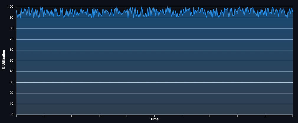
Then it may be far simpler, and possibly cheaper, to simply purchase reserved instances for 3 years. Or potentially, even just lease hardware directly and ignore the cloud.

Most banking HPC grids have utilisation that looks more like this:

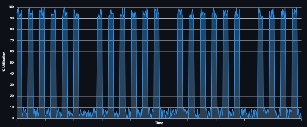
In this case, depending on the discounts you are able to secure with your cloud provider of choice, and what proportion of time the infrastructure is in use, it may be feasible to just use reserved instances. Though this is still potentially a case in which perhaps leased hardware is still cheaper.

If you happen to run any real-time risk analytics or other quasi real-time high throughput applications, it’s quite possible that your usage looks something like this:

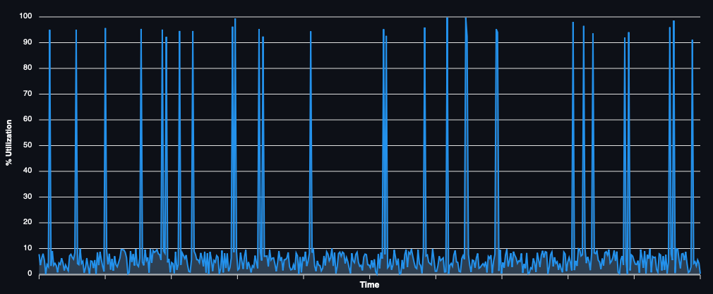
i.e. the darling of the cloud providers.

In this case, you are unlikely to use anything other than on-demand or spot due to the low percentage of time that the compute is required (perhaps with a far smaller quantity of reserved instances for the base load).

Having said that, as mentioned earlier, it’s quite likely that in all cases, the cheapest possible way to run your compute is using spot. Provided that you can deal with pre-emption and select the correct, most cost effective, VM type.

Performance Adjusted Pricing

In all cases, cloud compute capacity is sold as a price per hour (or month) for a given VM instance type. Comparing prices across different types of VMs can be done at best by using the number of CPUs (or memory) as a reference point (i.e. price per CPU).

However, as amply illustrated by our previous article, the performance of two different cloud VMs with the same CPU count can differ by a factor of 3. A price per CPU is hardly a useful metric given this knowledge.

Instead, it becomes much more valuable to compare VM pricing accounting for performance. Take two virtual machines A and B with the same number of CPUs and same amount of memory. Machine A performs three times faster than machine B but costs $0.01 per hour as opposed to machine B’s $0.005 per hour. Given machine B takes three times as long to perform the same amount of work as machine A, that gives us an effective price of $.0.015 per hour. Thus, making A the most cost-effective option despite the higher price and identical CPU count.

For this to be useful, the performance metric used must correlate well to your own workload. It is unlikely to be possible to have a single generally applicable performance adjusted price that can be compared across all use cases, but it is possible to have one for your own workload.

We use this approach in conjunction with the COREx (the financial risk HPC benchmark) results to calculate a COREx adjusted price.

Looking at the impact of price changes

The remainder of this article will focus on spot and on demand pricing only.

Let’s take our systemically important bank again as an example, with a monthly usage of 30 million CPU hours (globally), and let’s assume it’s split evenly across the USA, Europe and the Asia Pacific region. Being generous, let’s assume usage is 100% efficient with no wastage, and the bank operates entirely on cloud (yes, this is a little fanciful on both counts); 10 million CPU hours of compute in each geography per month.

In all the below examples, we have used publicly available prices. These may not reflect prices that large consumers of compute may be able to negotiate with the cloud providers (though generally, spot prices are not often discounted any further). The prices were current as of 26 June 2023.

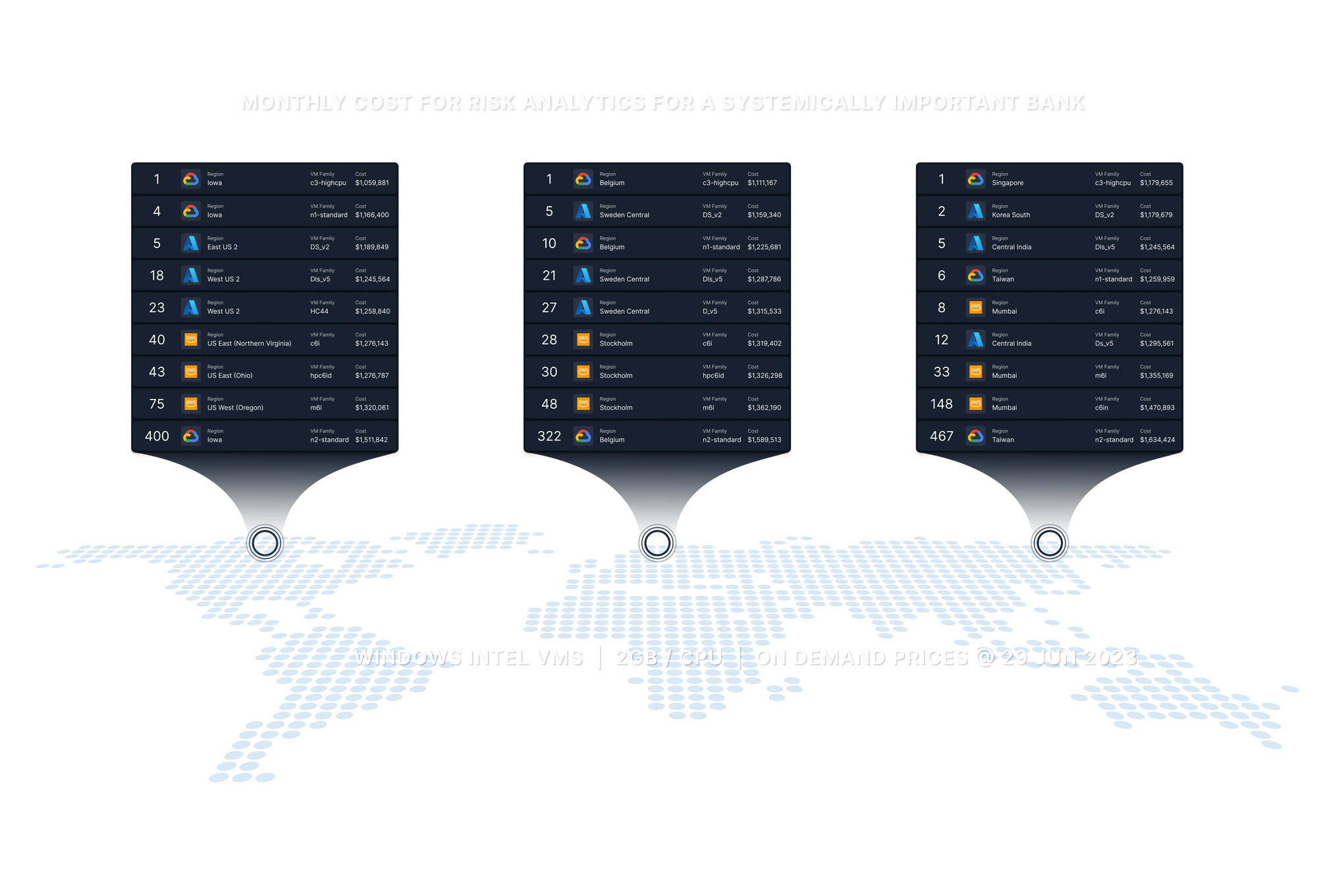
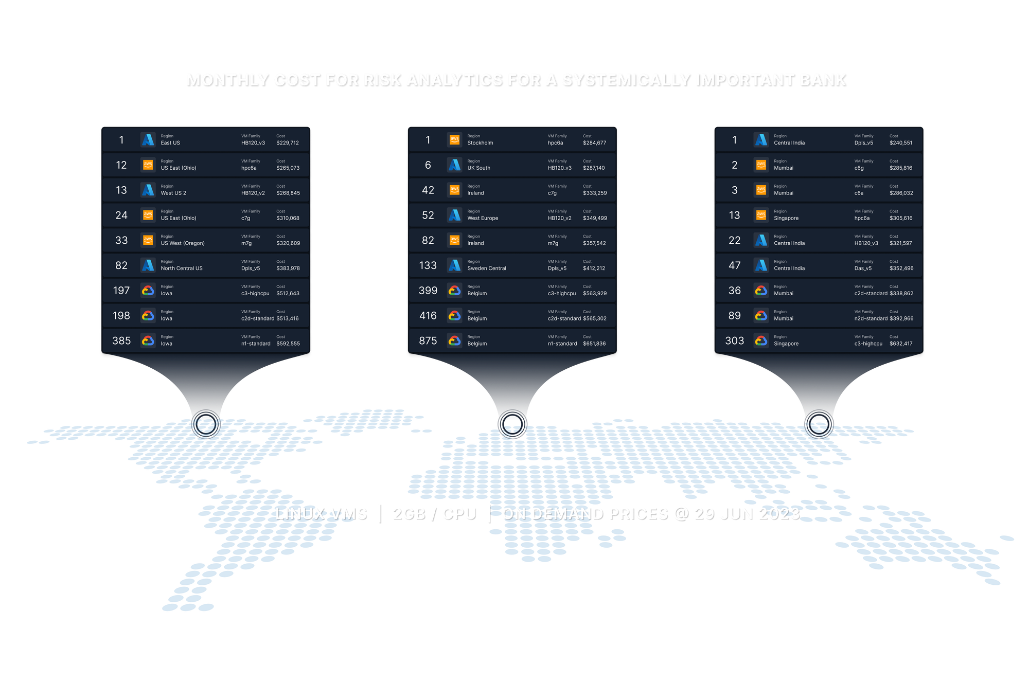
Example 1 — Windows & Intel Only

In the first example, suppose we have a bank that can run its analytics libraries only on Windows (not that uncommon) and has only certified them using Intel CPUs (again quite common). Being generous, let’s stipulate a requirement of a minimum of 2GB of RAM per CPU for the analytics to operate.

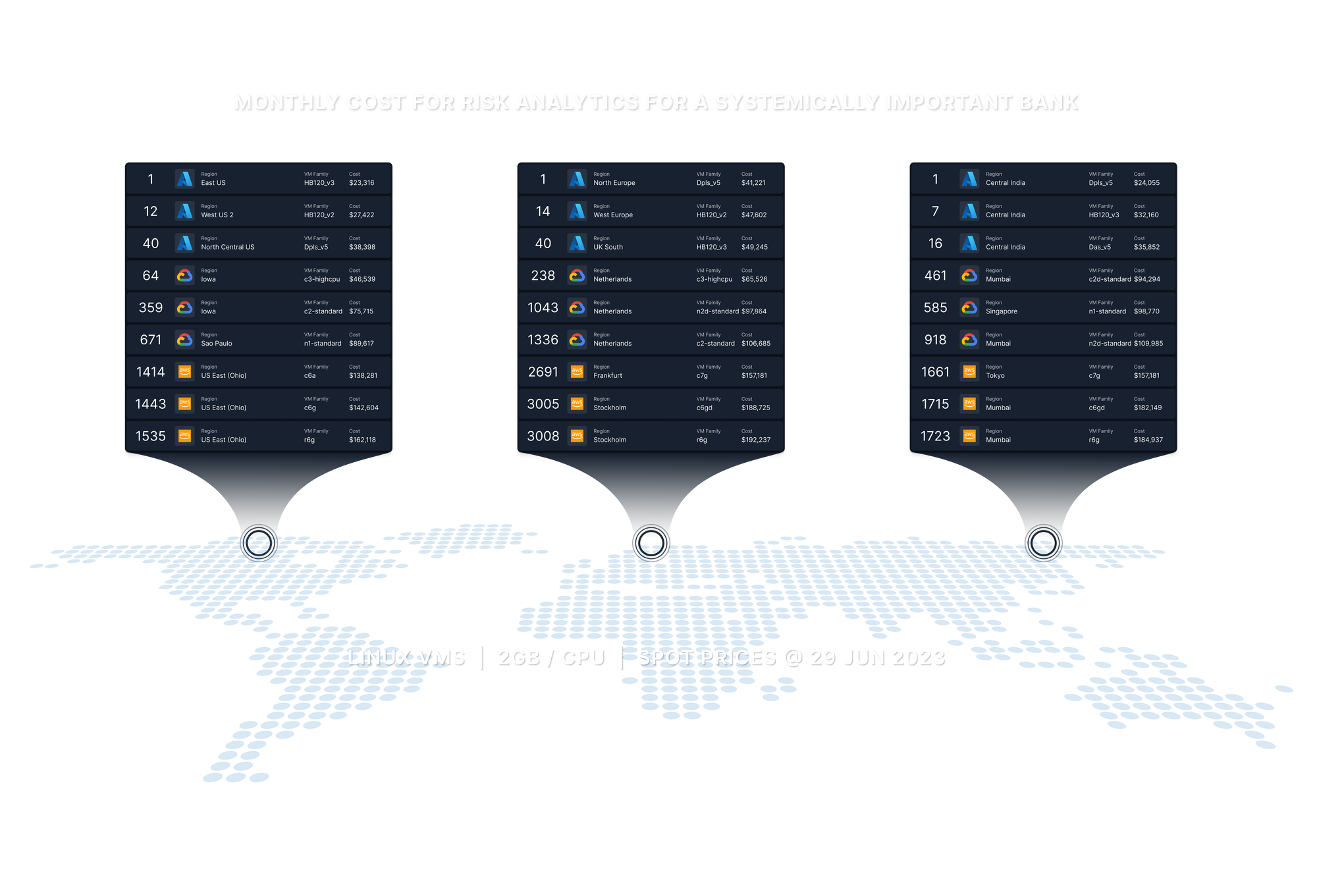
The cheapest three VM types which match these criteria and are in each of the three geographical regions from each of the three big cloud providers are listed below, in order of increasing COREx adjusted hourly cost per CPU. Often the same VM family will occupy consecutive positions (with multiple sizes of VM), in the interest of brevity and diversity in such cases instead of selecting the next cheapest VM type on the list, the next cheapest VM type of a different VM family is shown.

The total cost is based on the assumption that the entire 10 million CPU hours (per region) is run on the specified VM. The results are summarised in the following infographic

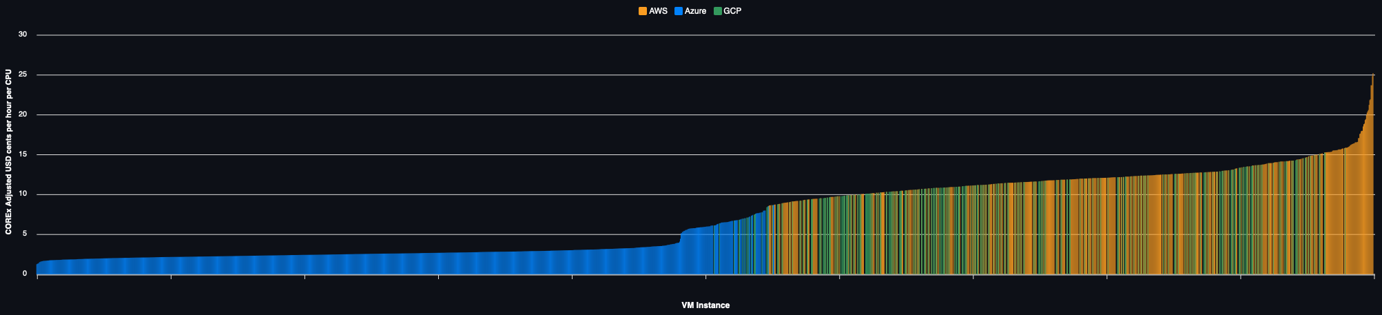
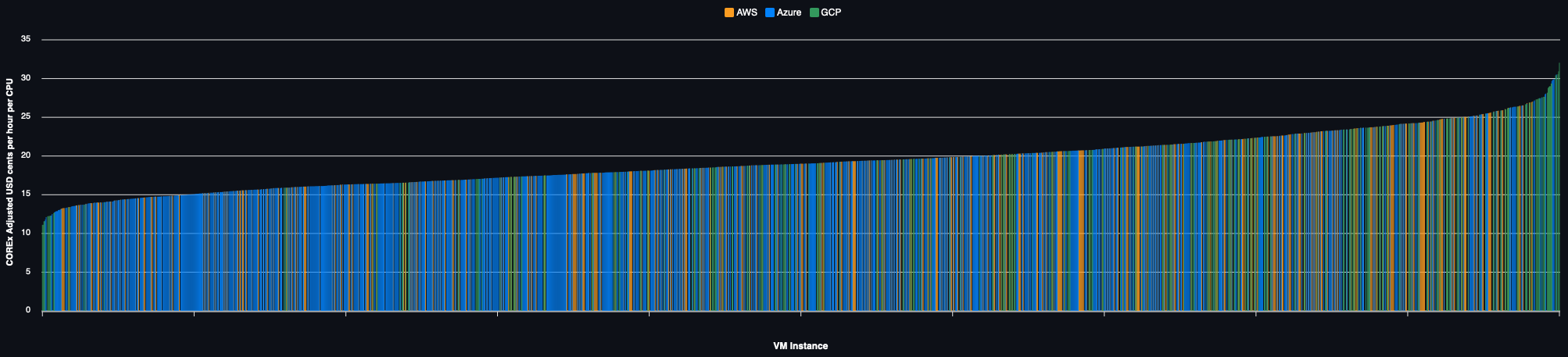
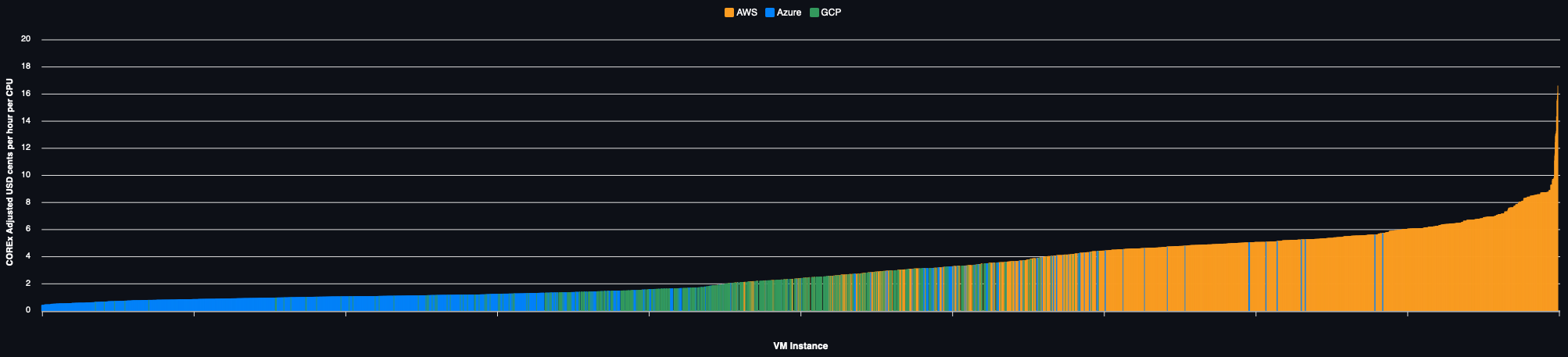
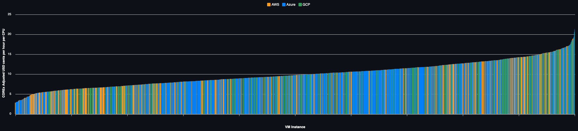
Spot Pricing

Alternatively, the performance adjusted price for each of the 650+ VMs in every region they are available are charted below for each region:

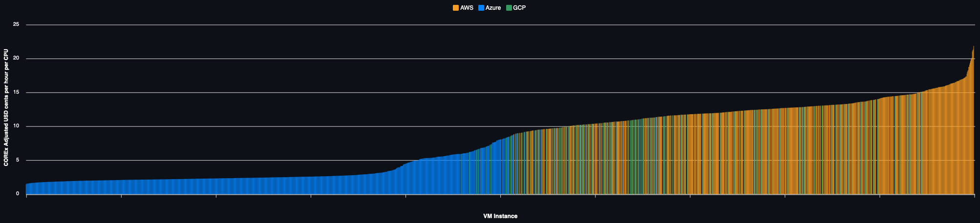
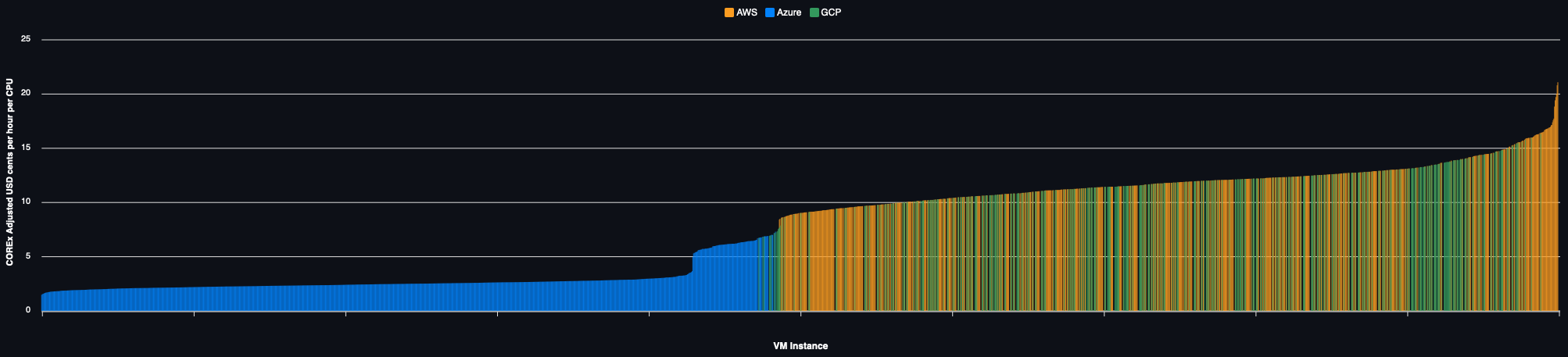
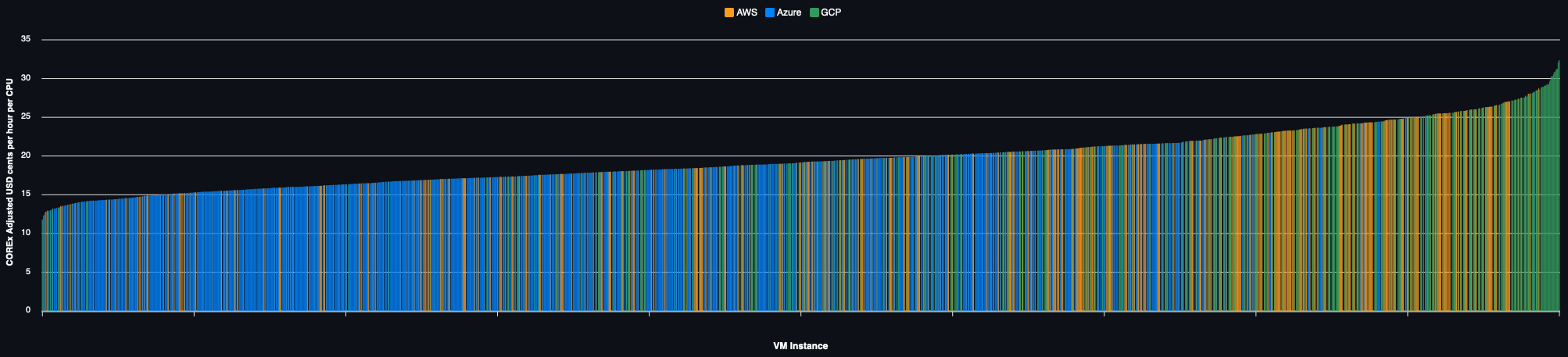
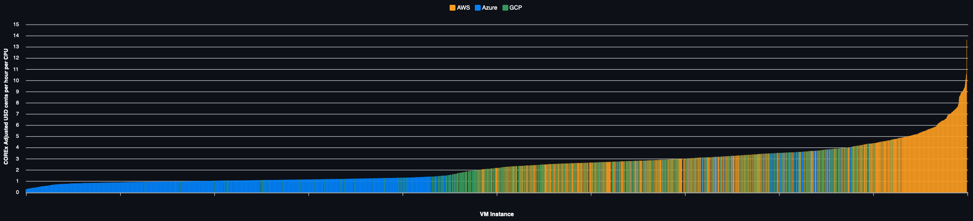
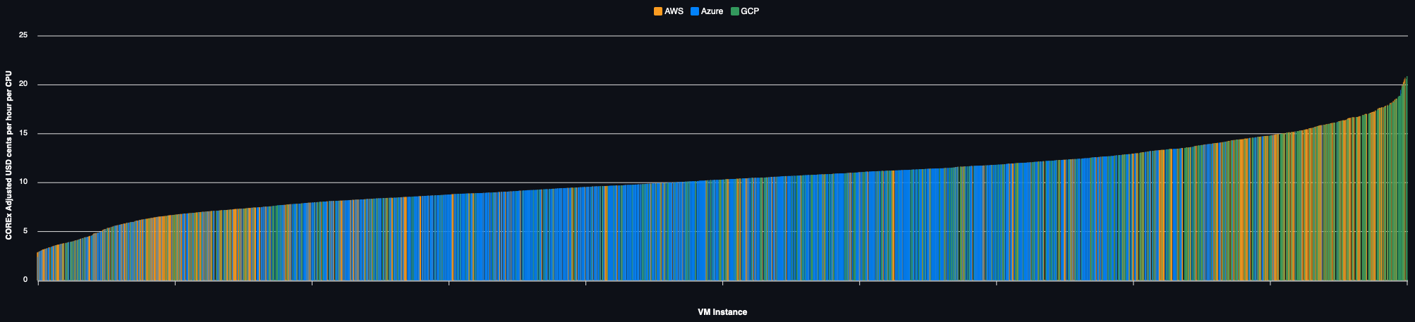
On Demand Pricing

Example 2 — Linux & Intel, AMD or ARM CPUs

A slightly less common scenario, assume a bank willing to run a non-premium OS (such as Debian or Ubuntu, i.e., no licensing costs) with analytics certified and optimised for use on any CPU architecture including ARM. We retain a memory to CPU ratio of 2GB per CPU and the same methodology as above for the infographic.

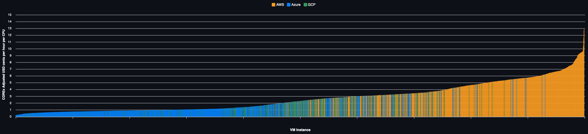
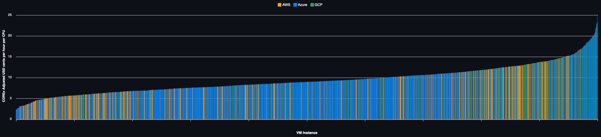
Spot Pricing

Regional prices for all VMs:

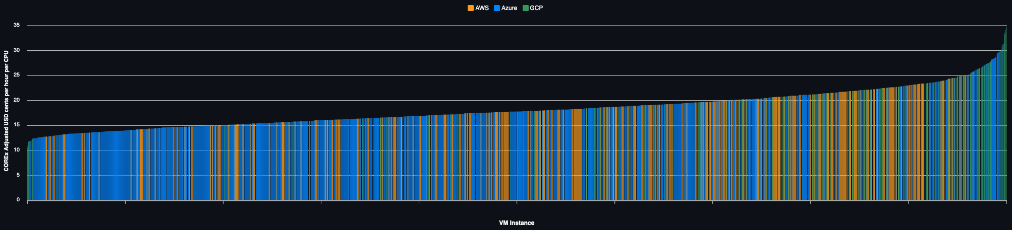
On Demand Pricing

The same example but using on demand capacity:

VM Type Selection

As is amply demonstrated above, the correct selection of not only the VM type but the region in which it is run can have a huge impact in the total cost of running HPC workloads.

Well optimised HPC systems would do well to select the optimal VM every time workload must be placed and spin up (and then down) on demand as the workload scales. At all times using the most cost effective VM, subject to operational constraints.

The process requires firstly the identification (or development) of a suitable benchmark which is reflective of your own workload (possibly more than one if there are multiple applications sharing an enterprise grid). COREx is a possible example of such a benchmark.

Assuming an appropriate benchmark is available (or COREx or Passmark are considered adequate), an API such as the following could be employed by a scheduler to provision the correct VM types

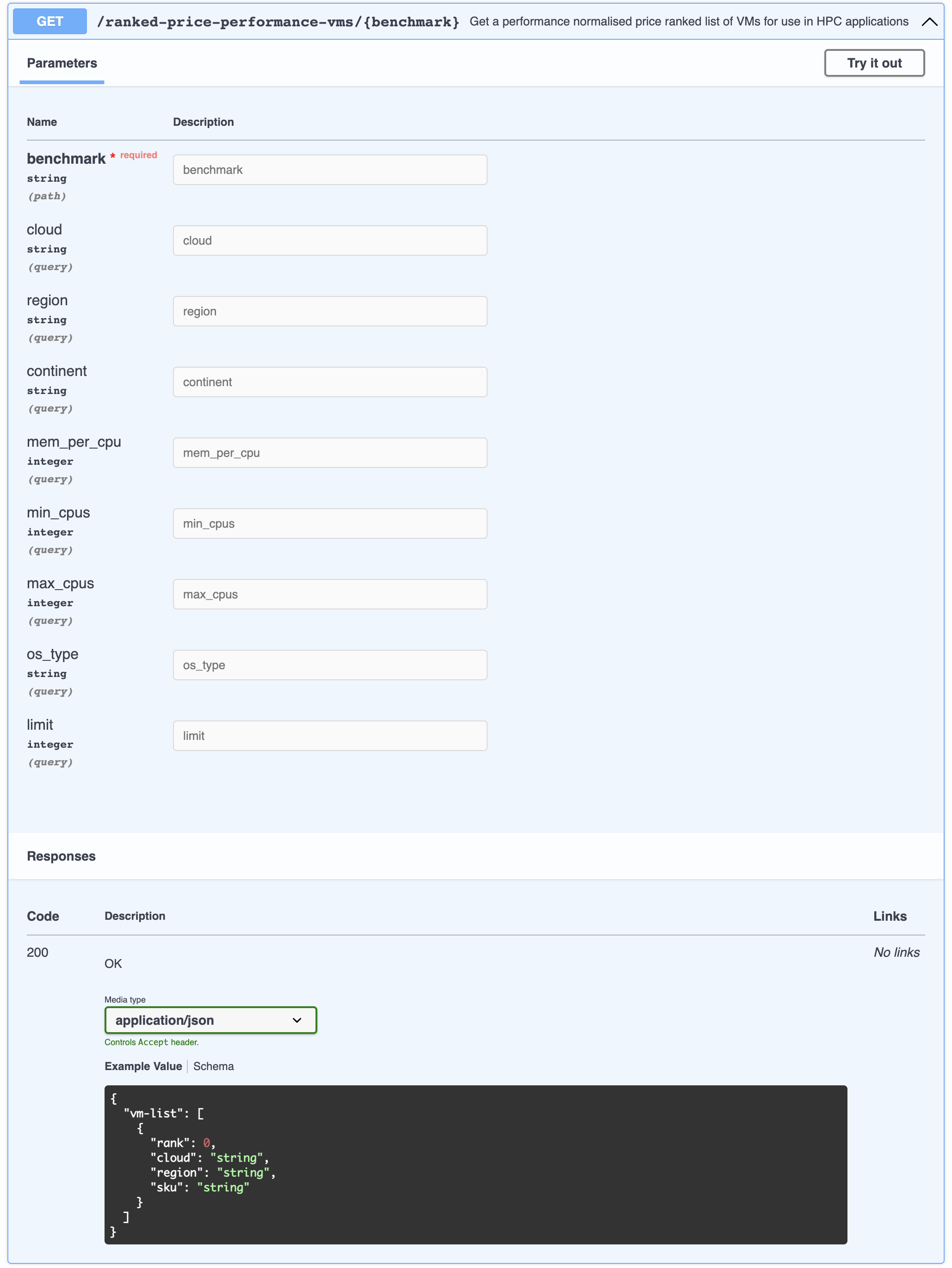
Whilst we may not yet be at a point where compute futures are traded on the CME, it is quite clear from the above, in order to fully optimize a HPC or HTC system, the scheduler must be able to exploit a variety of VM types across a number of regions and ideally even cloud providers. The potential cost savings speak for themselves. As do those for moving off a Windows and Intel only platform!

Interested in learning more? If the correct benchmark isn’t available, we’d always be happy to help you develop an appropriate test workload. Interested in using the above API? Why not get in touch?